3. Bias/variance tradeoff, mse, convergence, etc

import numpy as np
from scipy import stats
from itertools import product
from sklearn.linear_model import LinearRegression
from sklearn.neighbors import KNeighborsClassifier
from sklearn.ensemble import ExtraTreesClassifier
import scipy as sp
from tqdm import tqdm
import matplotlib.pylab as plt
import pandas as pd
%matplotlib inline

3.1. Bias/var/MSE of a linear regression coefficient

\(E_{\text{train}} (( \hat{\theta}_{\text{train}} - \theta )^2 ) = (E_{\text{train}} (\hat{\theta}_{\text{train}} - \theta ))^2 + \text{var}_{\text{train}} (\hat{\theta}_{\text{train}} - \theta ) = \text{bias}^2 + \text{variance}\)

np.random.seed(1)
true_beta = 1.3

def dataset_generator(size=200):
    x = np.random.random((size, 1))
    y = x.ravel() * true_beta + stats.norm().rvs(size)
    return x, y

# obtaining samples of distribution of estimated beta
est_beta = []
for i in tqdm(range(10000)):
    x, y = dataset_generator()
    est = LinearRegression().fit(x, y)
    est_beta.append(est.coef_.item())

est_beta = np.array(est_beta)

# measuring bias/var/mse of the linear regression **coefficient**:
bias = (est_beta - true_beta).mean()
var = est_beta.var()
mse_method1 = bias**2 + var
mse_method2 = ((est_beta - true_beta)**2).mean()
print('bias:', bias, '\nvar:', var, '\nmse_method1:', mse_method1, '\nmse_method2:', mse_method2)

100%|████████████████████████████████████| 10000/10000 [00:16<00:00, 607.64it/s]

bias: -0.0009472484975395509
var: 0.06002616178038994
mse_method1: 0.06002705906010603
mse_method2: 0.06002705906010603

3.2. Bias/var/MSE of a linear regression prediction on a specific point

\[\begin{split} \ \int_{y \in \mathbb{D|x_0}} \int_{D \in \mathbb{D}_{\text{train}}} ( \text{estimator}_{D}(x_0) - y )^2 \ d D \text{ } d y \ = \\ \ E_{\text{test}} \{ E_{\text{train}} \{ ( \text{estimator}_{\text{train}}(x_0) - y_{\text{test}}(x_0) )^2|D_{\text{test}} \}\} \ = \\ \ E_{\text{train}} \{ E_{\text{test}} \{ ( \text{estimator}_{\text{train}}(x_0) - y_{\text{test}}(x_0) )^2|D_{\text{train}} \}\} \ = \\ \ E_{\text{test}} \{ E_{\text{train}} \{ ( \text{estimator}_{\text{train}}(x_0) - y_{\text{test}}(x_0) )^2 \}\} \ = \\ \ (E_{\text{test}} \{ E_{\text{train}} \{ \text{estimator}_{\text{train}}(x_0) - y_{\text{test}}(x_0) \}\})^2 + \\ \ \text{var}_{\text{train}} \{ \text{estimator}_{\text{train}}(x_0) \} + \\ \ (E_{\text{test}} \{ E_{\text{train}} \{ ( y_{\text{train}}(x_0) - y_{\text{test}}(x_0) )^2 \}\})^2\ = \\ \ \text{bias}^2 + \text{variance} + \text{irreductible_error}\end{split}\]

\(E_{\text{train}}\): expectation over all possible dataset of fixed size (with the desired train dataset size).

\(E_{\text{test}}\): expectation over all possible samples of the data generating function.

np.random.seed(1)
def sample_y_given_x(x):
    y = x * true_beta + stats.norm().rvs(1).item()
    return y

# obtaining samples of distribution of estimated beta
est_y = []
true_y = []
for i in tqdm(range(10000)):
    x_train, y_train = dataset_generator()
    x_test = 0.35
    y_test = sample_y_given_x(x_test)

    est = LinearRegression().fit(x_train, y_train)
    est_y.append(est.predict(np.array([x_test]).reshape(1,1)))
    true_y.append(y_test)

est_y = np.hstack(est_y)
true_y = np.hstack(true_y)

# measuring bias/variance/mse of the linear regression **prediction**:
bias = (est_y - true_y).mean()
var = est_y.var()
partial_mse = bias**2 + var
full_mse = ((est_y - true_y)**2).mean()
irreductible_error = full_mse - partial_mse
print('bias:', bias, '\nvar:', var, '\npartial_mse:', partial_mse,
      '\nirreductible_error:', irreductible_error, '\nfull_mse:', full_mse)

100%|████████████████████████████████████| 10000/10000 [00:20<00:00, 487.10it/s]

bias: 0.028075696825567296
var: 0.006434741506324545
partial_mse: 0.007222986258565715
irreductible_error: 1.003423201725877
full_mse: 1.0106461879844428

3.3. Bias/var/MSE of a linear regression prediction integrated on χ

\[\begin{split} \ \int_{(y,x) \in \mathbb{D}} \int_{D \in \mathbb{D}_{\text{train}}} ( \text{estimator}_{D}(x) - y )^2 \ d D \text{ } d (y,x) \ = \\ \ E_{\text{test}} \{ E_{\text{train}} \{ ( \text{estimator}_{\text{train}}(x_{\text{test}}) - y_{\text{test}}(x_{\text{test}}) )^2 \}\} \ = \\ \ (E_{\text{test}} \{ E_{\text{train}} \{ \text{estimator}_{\text{train}}(x_{\text{test}}) - y_{\text{test}}(x_{\text{test}}) \}\})^2 + \\ \ E_{\text{test}} \{ \text{var}_{\text{train}} \{ \text{estimator}_{\text{train}}(x_{\text{test}}) \}\} + \\ \ (E_{\text{test}} \{ E_{\text{train}} \{ ( y_{\text{train}}(x_{\text{test}}) - y_{\text{test}}(x_{\text{test}}) )^2 \}\})^2\ = \\ \ \text{bias}^2 + \text{variance} + \text{irreductible_error}\end{split}\]

np.random.seed(1)
# obtaining samples of distribution of estimated beta
n_experiments = 10_000
n_test_db = 30_000

x_test, y_test = dataset_generator(n_test_db)
est_y = np.empty((n_test_db, n_experiments))

true_y = y_test.reshape((-1,1))
for i in tqdm(range(n_experiments)):
    x_train, y_train = dataset_generator()

    est = LinearRegression().fit(x_train, y_train)
    est_y[:, i] = est.predict(x_test)

# measuring bias/variance/mse of the linear regression **prediction**:
bias = (est_y - true_y).mean()
bias_ste = bias.std()
var = est_y.var(1).mean()
partial_mse = bias**2 + var
full_mse = ((est_y - true_y)**2).mean()
irreductible_error = full_mse - partial_mse
print('bias:', bias, '\nvar:', var, '\npartial_mse:', partial_mse,
      '\nirreductible_error:', irreductible_error, '\nfull_mse:', full_mse)

100%|████████████████████████████████████| 10000/10000 [00:14<00:00, 692.91it/s]

bias: -0.0020629011362093856
var: 0.010069500001760602
partial_mse: 0.010073755562858376
irreductible_error: 1.0028603529185194
full_mse: 1.0129341084813777

# Bonus, let's get the confidence intervals using the delta method!
# https://en.wikipedia.org/wiki/Delta_method

bias_arr = (est_y - true_y).mean(1)
bias_mean = bias_arr.mean()
bias_se = bias_arr.std() / np.sqrt(len(bias_arr))
bias_dist = stats.norm(bias_mean, bias_se)

var_arr = est_y.var(1)
var_mean = var_arr.mean()
var_se = var_arr.std() / np.sqrt(len(var_arr))
var_dist = stats.norm(var_mean, var_se)

cov = np.cov(bias_arr, var_arr)
partial_mse_mean = bias_mean**2 + var_mean
partial_mse_se = np.matmul([2*bias_mean, 1], cov)
partial_mse_se = np.matmul(partial_mse_se, [[2*bias_mean], [1]])
partial_mse_se = partial_mse_se.item() / np.sqrt(len(var_arr))
partial_mse_dist = stats.norm(partial_mse_mean, partial_mse_se)

full_mse_arr = ((est_y - true_y)**2).mean(1)
full_mse_mean = full_mse_arr.mean()
full_mse_se = full_mse_arr.std() / np.sqrt(len(full_mse_arr))
full_mse_dist = stats.norm(full_mse_mean, full_mse_se)

cov = np.cov(np.vstack([full_mse_arr, bias_arr, var_arr]))
irreductible_error_mean = full_mse_mean - bias_mean**2 - var_mean
irreductible_error_se = np.matmul([1, -2*bias_mean, -1], cov)
irreductible_error_se = np.matmul(irreductible_error_se, [[1], [-2*bias_mean], [-1]])
irreductible_error_se = irreductible_error_se.item() / np.sqrt(len(var_arr))
irreductible_error_dist = stats.norm(irreductible_error_mean, irreductible_error_se)

print(f'P(bias ∈ [{np.round(bias_dist.ppf(0.01), 4)}, {np.round(bias_dist.ppf(0.99), 4)}]) >= 0.99')
print(f'P(var ∈ [{np.round(var_dist.ppf(0.01), 4)}, {np.round(var_dist.ppf(0.99), 4)}]) >= 0.99')
print(f'P(partial_mse ∈ [{np.round(partial_mse_dist.ppf(0.01), 4)}, {np.round(partial_mse_dist.ppf(0.99), 4)}]) >= 0.99')
print(f'P(irreductible_error ∈ [{np.round(irreductible_error_dist.ppf(0.01), 4)}, {np.round(irreductible_error_dist.ppf(0.99), 4)}]) >= 0.9')
print(f'P(full_mse ∈ [{np.round(full_mse_dist.ppf(0.01), 4)}, {np.round(full_mse_dist.ppf(0.99), 4)}]) >= 0.99')

P(bias ∈ [-0.0155, 0.0114]) >= 0.99
P(var ∈ [0.01, 0.0101]) >= 0.99
P(partial_mse ∈ [0.0101, 0.0101]) >= 0.99
P(irreductible_error ∈ [0.9756, 1.0301]) >= 0.9
P(full_mse ∈ [0.9938, 1.0321]) >= 0.99

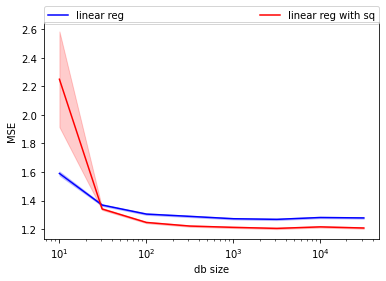
3.4. MSE of a linear regression with and without a quadratic term

def dataset_generator_2(size=30):
    x = np.random.random((size, 1))
    y = x.ravel() * 1.78 + x.ravel()**2 * 3.5 + stats.norm(0,1.1).rvs(size)
    return x, y

print("Irreductible error:", stats.norm(0,1.1).var())

Irreductible error: 1.2100000000000002

np.random.seed(1)
mse_lin_nsq = []
mse_lin_nsq_stderr = []
mse_lin_wsq = []
mse_lin_wsq_stderr = []
mse_svr = []
db_sizes = np.array(10**np.arange(1.,5.,0.5),dtype=int)

for db_size in tqdm(db_sizes):
    se = []
    for i in range(3000):
        x_train, y_train = dataset_generator_2(db_size)
        x_test, y_test = dataset_generator_2(100)

        est = LinearRegression().fit(x_train, y_train)
        pred = est.predict(x_test)
        se.append(((pred-y_test)**2).mean())
    mse_lin_nsq.append(np.mean(se))
    mse_lin_nsq_stderr.append(np.std(se)/np.sqrt(len(se)))

for db_size in tqdm(db_sizes):
    se = []
    for i in range(3000):
        x_train, y_train = dataset_generator_2(db_size)
        x_test, y_test = dataset_generator_2(100)

        est = LinearRegression().fit(np.hstack([x_train, x_train**2]), y_train)
        pred = est.predict(np.hstack([x_test, x_test**2]))
        se.append(((pred-y_test)**2).mean())
    mse_lin_wsq.append(np.mean(se))
    mse_lin_wsq_stderr.append(np.std(se)/np.sqrt(len(se)))

100%|█████████████████████████████████████████████| 8/8 [00:43<00:00,  5.43s/it]
100%|█████████████████████████████████████████████| 8/8 [00:47<00:00,  5.92s/it]

plt.plot(db_sizes, mse_lin_nsq, color='blue', label="linear reg")
plt.fill_between(db_sizes,
                 stats.norm(mse_lin_nsq, mse_lin_nsq_stderr).ppf(0.05),
                 stats.norm(mse_lin_nsq, mse_lin_nsq_stderr).ppf(0.95),
                 alpha=0.2, color='blue')

plt.plot(db_sizes, mse_lin_wsq, color='red', label="linear reg with sq")
plt.fill_between(db_sizes,
                 stats.norm(mse_lin_wsq, mse_lin_wsq_stderr).ppf(0.05),
                 stats.norm(mse_lin_wsq, mse_lin_wsq_stderr).ppf(0.95),
                 alpha=0.2, color='red')

plt.xlabel("db size")
plt.ylabel("MSE")
plt.legend(bbox_to_anchor=(0, 1.07, 1, 0), mode="expand", ncol=3, borderaxespad=0.)
plt.semilogx(base=10);

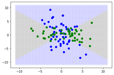
3.5. Bayes Error Rate of classifier

np.random.seed(12)
true_beta = stats.norm(0).rvs((2,1))

def gen_db(x):
    y = np.matmul(x**2, true_beta).ravel()
    y_prob = sp.special.expit(y)
    y = stats.bernoulli(y_prob).rvs()
    return y, y_prob

# test sample
x = np.linspace(-11,11,250)
x = product(x,x)
x = np.array(list(x))
y, y_prob = gen_db(x)
y_pred = y_prob > 0.5
plt.scatter(x[y_pred==0,0], x[y_pred==0,1], alpha=0.005, color='blue')
plt.scatter(x[y_pred==1,0], x[y_pred==1,1], alpha=0.005, color='green')

x = stats.norm(0,3).rvs((100,2))
y, y_prob = gen_db(x)
y_pred = y_prob > 0.5
plt.scatter(x[y==0,0], x[y==0,1], color='blue')
plt.scatter(x[y==1,0], x[y==1,1], color='green')

x = stats.norm(0,3).rvs((10000,2))
y, y_prob = gen_db(x)
y_pred = y_prob > 0.5
print("Bayes error rate:", (y != y_pred).mean(), "+-", 3*(y != y_pred).std()/np.sqrt(len(y)))

Bayes error rate: 0.1281 +- 0.010026033662421047

np.random.seed(1)
true_beta = stats.norm().rvs((5,1), random_state=1)

def gen_x(size):
    x = np.random.random((size, 5))
    return x

def gen_y_given_x(x):
    y = np.matmul(x, true_beta).ravel()

    # noise generator
    y = y + stats.norm(0., 1.3).rvs(len(x))

    y = y >= 0
    return y+0

def get_y_prob_given_x(x):
    y_prob = np.empty(len(x))+np.nan
    for i in range(len(x)):
        y_prob[i] = gen_y_given_x(np.zeros((10_000, len(x[i]))) + x[i]).mean()
    return y_prob

# test sample
x = gen_x(2_000)
y = gen_y_given_x(x)

# best possible classifier
y_prob = get_y_prob_given_x(x)
y_pred = y_prob > 0.5

print("Bayes error rate:", (y != y_pred).mean(), "+-", 3*(y != y_pred).std()/np.sqrt(len(y)))
print("Irreductible KS:", stats.ks_2samp(y_prob[y==0], y_prob[y==1]).statistic)

Bayes error rate: 0.33 +- 0.03154282802793688
Irreductible KS: 0.35013682351181696

np.random.seed(1)
x_train = gen_x(2_000)
y_train = gen_y_given_x(x_train)
x_test = gen_x(2_000)
y_test = gen_y_given_x(x_test)

est = ExtraTreesClassifier().fit(x_train, y_train)
y_pred = est.predict_proba(x_test)

zo_loss = (y_test != np.argmax(y_pred, 1)).mean()
ks = stats.ks_2samp(y_pred[y_test==0,1], y_pred[y_test==1,1]).statistic

print("Zero-one loss:", zo_loss)
print("KS:", ks)

Zero-one loss: 0.376
KS: 0.2656788574232497

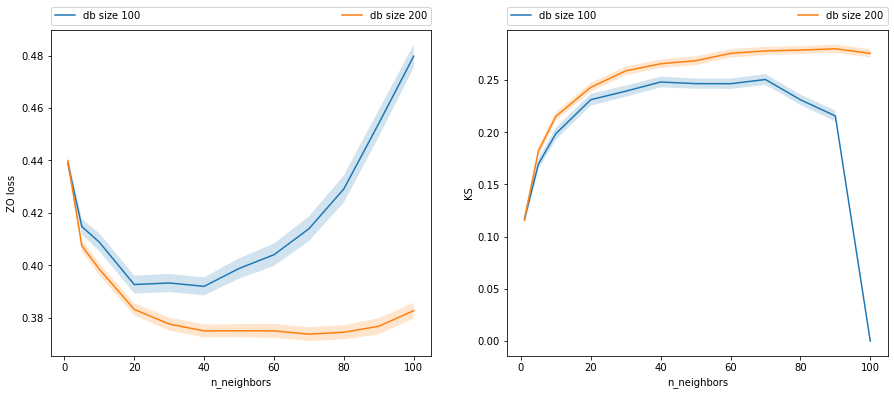
3.6. Complexity and sample size on a KNN

np.random.seed(1)
db_sizes = [100, 200]

df = []
for db_size in db_sizes:
    for n_neighbors in tqdm([1, 5, 10, 20, 30, 40, 50, 60, 70, 80, 90, 100]):
        # obtaining samples of distribution of estimated beta

        zo = []
        ks = []
        for i in range(200):
            x_train = gen_x(db_size)
            y_train = gen_y_given_x(x_train)
            x_test = gen_x(1_000)
            y_test = gen_y_given_x(x_test)

            est = KNeighborsClassifier(n_neighbors).fit(x_train, y_train)
            y_pred = est.predict_proba(x_test)

            zo.append((y_test != np.argmax(y_pred, 1)).mean())
            ks.append(stats.ks_2samp(y_pred[y_test==0,1], y_pred[y_test==1,1]).statistic)

        res = dict(db_size=db_size, n_neighbors=n_neighbors)
        res['zo_mean'] = np.mean(zo)
        res['zo_se'] = np.std(zo) / np.sqrt(len(zo))
        res['ks_mean'] = np.mean(ks)
        res['ks_se'] = np.std(ks) / np.sqrt(len(ks))
        df.append(res)

df = pd.DataFrame(df)

100%|███████████████████████████████████████████| 12/12 [00:25<00:00,  2.15s/it]
100%|███████████████████████████████████████████| 12/12 [00:30<00:00,  2.57s/it]

_, axes = plt.subplots(1,2, figsize=(15,6))
for db_size in df.db_size.unique():
    dff = df[df.db_size==db_size]

    plt.sca(axes[0])
    plt.plot(dff.n_neighbors, dff.zo_mean, label=f"db size {db_size}")
    plt.fill_between(dff.n_neighbors,
                     stats.norm(dff.zo_mean, dff.zo_se).ppf(0.05),
                     stats.norm(dff.zo_mean, dff.zo_se).ppf(0.95),
                     alpha=0.2)
    plt.xlabel("n_neighbors")
    plt.ylabel("ZO loss")
    plt.legend(bbox_to_anchor=(0, 1.07, 1, 0), mode="expand", ncol=3, borderaxespad=0.)

    plt.sca(axes[1])
    plt.plot(dff.n_neighbors, dff.ks_mean, label=f"db size {db_size}")
    plt.fill_between(dff.n_neighbors,
                     stats.norm(dff.ks_mean, dff.ks_se).ppf(0.05),
                     stats.norm(dff.ks_mean, dff.ks_se).ppf(0.95),
                     alpha=0.2)

    plt.xlabel("n_neighbors")
    plt.ylabel("KS")
    plt.legend(bbox_to_anchor=(0, 1.07, 1, 0), mode="expand", ncol=3, borderaxespad=0.)

/home/marco/miniforge3/lib/python3.8/site-packages/scipy/stats/_distn_infrastructure.py:2023: RuntimeWarning: invalid value encountered in multiply
  lower_bound = _a * scale + loc
/home/marco/miniforge3/lib/python3.8/site-packages/scipy/stats/_distn_infrastructure.py:2024: RuntimeWarning: invalid value encountered in multiply
  upper_bound = _b * scale + loc

3.7. Measuring the quality of a classifier using a holdout set

One question remains, what are we estimating we when create a error prediction interval using a holdout set? Are we estimating the Loss of the estimator for that data generating function? i.e.:

\[E_{\text{test}} \{ E_{\text{train}} \{ \text{Loss}( \text{estimator}_{\text{train}}(x_{\text{test}}), y_{\text{test}}(x_{\text{test}}) ) \}\}\]

Let’s try it out, first let’s get a very accurate estimate of this using the replication of experiments method:

np.random.seed(1)
zo = []
ks = []
for i in tqdm(range(20000)):
    x_train = gen_x(100)
    y_train = gen_y_given_x(x_train)
    x_test = gen_x(1_000)
    y_test = gen_y_given_x(x_test)

    est = KNeighborsClassifier(10).fit(x_train, y_train)
    y_pred = est.predict_proba(x_test)

    zo.append((y_test != np.argmax(y_pred, 1)).mean())
    ks.append(stats.ks_2samp(y_pred[y_test==0,1], y_pred[y_test==1,1]).statistic)

zo_mean_app = np.mean(zo)
zo_se = np.std(zo) / np.sqrt(len(zo))
ks_mean_app = np.mean(ks)
ks_se = np.std(ks) / np.sqrt(len(ks))
zo_mean_app, zo_se, ks_mean_app, ks_se

100%|████████████████████████████████████| 20000/20000 [02:36<00:00, 127.47it/s]

(0.40653925,
 0.00019486239496597336,
 0.20277423445795634,
 0.0003380796529185385)

Now, let’s obtain confidence intervals using holdout set and check how often they contain the "true" value of for the ZO-LOSS

np.random.seed(1)
contained = []
pbar = tqdm(range(1000))
for i in pbar:
    zo = []
    ks = []
    x_train = gen_x(100)
    y_train = gen_y_given_x(x_train)
    x_test = gen_x(1_000)
    y_test = gen_y_given_x(x_test)

    est = KNeighborsClassifier(10).fit(x_train, y_train)
    y_pred = est.predict_proba(x_test)

    zo = (y_test != np.argmax(y_pred, 1))
    zo_mean = np.mean(zo)
    zo_se = np.std(zo) / np.sqrt(len(zo))

    ci_interval_lower = stats.norm(zo_mean, zo_se).ppf(0.05)
    ci_interval_upper = stats.norm(zo_mean, zo_se).ppf(0.95)

    contained.append(ci_interval_lower <= zo_mean_app and zo_mean_app <= ci_interval_upper)
    pbar.set_description(f"Coverage {np.mean(contained)}")

Coverage 0.632: 100%|██████████████████████| 1000/1000 [00:06<00:00, 142.86it/s]

This low coverage is a symptom that we are not actually estimating that, but rather the loss of that particular trained estimator on the true data generating function:

\[E_{\text{test}} \{ \text{Loss}( \text{estimator}_{\text{train}}(x_{\text{test}}), y_{\text{test}}(x_{\text{test}}) ) | D_{\text{train}} \}\]

np.random.seed(1)
contained = []
pbar = tqdm(range(1000))
for i in pbar:
    zo = []
    ks = []
    x_train = gen_x(100)
    y_train = gen_y_given_x(x_train)

    x_test = gen_x(1_000)
    y_test = gen_y_given_x(x_test)

    x_production = gen_x(100_000)
    y_production = gen_y_given_x(x_production)

    est = KNeighborsClassifier(10).fit(x_train, y_train)
    y_pred = est.predict_proba(x_test)

    zo = (y_test != np.argmax(y_pred, 1))
    zo_mean = np.mean(zo)
    zo_se = np.std(zo) / np.sqrt(len(zo))

    y_pred_production = est.predict_proba(x_production)
    zo_production = (y_production != np.argmax(y_pred_production, 1)).mean()

    ci_interval_lower = stats.norm(zo_mean, zo_se).ppf(0.05)
    ci_interval_upper = stats.norm(zo_mean, zo_se).ppf(0.95)

    contained.append(ci_interval_lower <= zo_production and zo_production <= ci_interval_upper)
    pbar.set_description(f"Coverage {np.mean(contained)}")

Coverage 0.907: 100%|███████████████████████| 1000/1000 [04:06<00:00,  4.06it/s]