5. Matploblib

Matplotlib is without much doubt the most well known and used Python library when the matter is 2D plots.

The easiest and simplest way to use matplotlib is by using its pyplot "interface":

import matplotlib.pyplot as plt

If you are using a Jupyter notebook, then you might want to run

%matplotlib inline

This will make the plots embeed in you Jupyter notebook.

If you are using an Ipython console, then run %matplotlib to have matplotlib work in an interactive-friendly way.

Otherwise, you will need to run plt.show() after each plot in this tutorial.

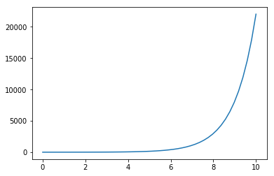
Now that you are setup, let’s run a simple example:

import numpy as np
x = np.linspace(0, 10)
y = np.exp(x)
plt.plot(x, y)

[<matplotlib.lines.Line2D at 0x7f8e640a9550>]

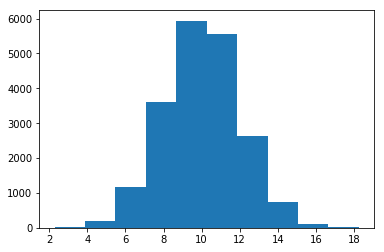
Here’s a simple histogram:

import scipy.stats as stats
x = stats.norm.rvs(loc=10, scale=2, size=20000)
plt.hist(x)

(array([  14.,  209., 1173., 3621., 5938., 5549., 2642.,  729.,  116.,
           9.]),
 array([ 2.27737477,  3.87540857,  5.47344237,  7.07147617,  8.66950997,
        10.26754377, 11.86557757, 13.46361137, 15.06164517, 16.65967897,
        18.25771277]),
 <a list of 10 Patch objects>)

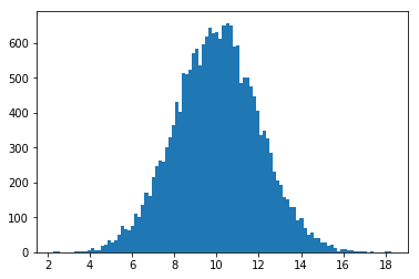
And another histogram of x with more bins:

plt.hist(x, 100)

(array([  1.,   1.,   0.,   0.,   0.,   0.,   1.,   4.,   3.,   4.,   5.,
         12.,   5.,   7.,  17.,  20.,  34.,  27.,  33.,  49.,  74.,  65.,
         62.,  75., 111., 102., 136., 171., 162., 215., 246., 264., 261.,
        300., 330., 365., 431., 402., 512., 510., 523., 570., 584., 537.,
        596., 617., 644., 626., 630., 611., 650., 657., 650., 589., 594.,
        485., 502., 500., 476., 446., 405., 335., 348., 325., 286., 231.,
        207., 194., 159., 152., 129., 131.,  92.,  97.,  68.,  50.,  55.,
         40.,  40.,  27.,  28.,  19.,  22.,  11.,   3.,  10.,   9.,   6.,
          5.,   3.,   3.,   1.,   2.,   0.,   1.,   0.,   0.,   0.,   1.,
          1.]),
 array([ 2.27737477,  2.43717815,  2.59698153,  2.75678491,  2.91658829,
         3.07639167,  3.23619505,  3.39599843,  3.55580181,  3.71560519,
         3.87540857,  4.03521195,  4.19501533,  4.35481871,  4.51462209,
         4.67442547,  4.83422885,  4.99403223,  5.15383561,  5.31363899,
         5.47344237,  5.63324575,  5.79304913,  5.95285251,  6.11265589,
         6.27245927,  6.43226265,  6.59206603,  6.75186941,  6.91167279,
         7.07147617,  7.23127955,  7.39108293,  7.55088631,  7.71068969,
         7.87049307,  8.03029645,  8.19009983,  8.34990321,  8.50970659,
         8.66950997,  8.82931335,  8.98911673,  9.14892011,  9.30872349,
         9.46852687,  9.62833025,  9.78813363,  9.94793701, 10.10774039,
        10.26754377, 10.42734715, 10.58715053, 10.74695391, 10.90675729,
        11.06656067, 11.22636405, 11.38616743, 11.54597081, 11.70577419,
        11.86557757, 12.02538095, 12.18518433, 12.34498771, 12.50479109,
        12.66459447, 12.82439785, 12.98420123, 13.14400461, 13.30380799,
        13.46361137, 13.62341475, 13.78321813, 13.94302151, 14.10282489,
        14.26262827, 14.42243165, 14.58223503, 14.74203841, 14.90184179,
        15.06164517, 15.22144855, 15.38125193, 15.54105531, 15.70085869,
        15.86066207, 16.02046545, 16.18026883, 16.34007221, 16.49987559,
        16.65967897, 16.81948235, 16.97928573, 17.13908911, 17.29889249,
        17.45869587, 17.61849925, 17.77830263, 17.93810601, 18.09790939,
        18.25771277]),
 <a list of 100 Patch objects>)

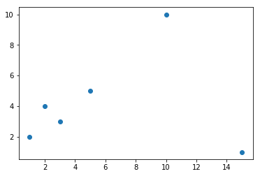
An scatter plot is also a piece of cake:

x = np.array([1, 2, 3, 5, 10, 15])
y = np.array([2, 4, 3, 5, 10, 1])
plt.scatter(x,y)
plt.show()

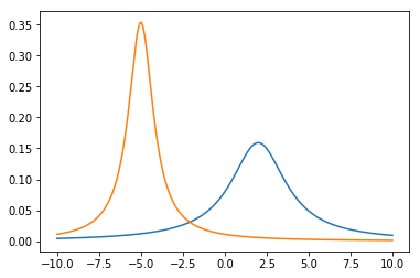
With multiple calls to method plot, you can have multiple curves in the same plot too:

x = np.linspace(-10, 10, 10000)
y1 = stats.cauchy.pdf(x, loc=2, scale=2)
y2 = stats.cauchy.pdf(x, loc=-5, scale=0.9)
plt.plot(x, y1)
plt.plot(x, y2)

[<matplotlib.lines.Line2D at 0x7f8e5bad3780>]

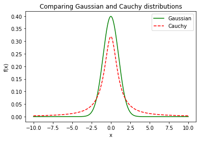
Adding legend and title is also a piece of cake:

x = np.linspace(-10, 10, 10000)
y1 = stats.norm.pdf(x, loc=0, scale=1)
y2 = stats.cauchy.pdf(x, loc=0, scale=1)
plt.plot(x, y1, label="Gaussian", color="green")
plt.plot(x, y2, label="Cauchy", color="red", linestyle='--')
plt.xlabel('x')
plt.ylabel('f(x)')
plt.title('Comparing Gaussian and Cauchy distributions')
plt.legend()

<matplotlib.legend.Legend at 0x7f8e5ba220b8>

It also possible to have multiple plots (subplots) inside a single plot:

plt.subplot(2, 1, 1)
plt.plot(x, y1, color="green")
plt.subplot(2, 1, 2)
plt.plot(x, y2, color="red", linestyle='--')

[<matplotlib.lines.Line2D at 0x7f8e5b998e10>]

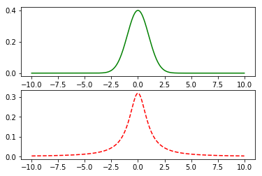
Here we pass the number of rows as the first parameter of method subplot, the number os columns as the second and activation (position, try inverting them) as the third.