2. Time series analysis
[1]:
import numpy as np
import pandas as pd
import scipy.stats as stats
from sklearn import metrics
from sklearn.model_selection import train_test_split
import os
import scipy.stats as stats
import matplotlib.pylab as plt
from collections import Counter
from datetime import datetime
import statsmodels as sm
import statsmodels.api as sma
from tqdm import tqdm
import catboost as catb

%matplotlib inline
[2]:
# Download dataset at https://www.kaggle.com/rohitsahoo/sales-forecasting
df = pd.read_csv('supersales_train.csv')
[3]:
df.head()
[3]:
| Row ID | Order ID | Order Date | Ship Date | Ship Mode | Customer ID | Customer Name | Segment | Country | City | State | Postal Code | Region | Product ID | Category | Sub-Category | Product Name | Sales | |
|---|---|---|---|---|---|---|---|---|---|---|---|---|---|---|---|---|---|---|
| 0 | 1 | CA-2017-152156 | 08/11/2017 | 11/11/2017 | Second Class | CG-12520 | Claire Gute | Consumer | United States | Henderson | Kentucky | 42420.0 | South | FUR-BO-10001798 | Furniture | Bookcases | Bush Somerset Collection Bookcase | 261.9600 |
| 1 | 2 | CA-2017-152156 | 08/11/2017 | 11/11/2017 | Second Class | CG-12520 | Claire Gute | Consumer | United States | Henderson | Kentucky | 42420.0 | South | FUR-CH-10000454 | Furniture | Chairs | Hon Deluxe Fabric Upholstered Stacking Chairs,... | 731.9400 |
| 2 | 3 | CA-2017-138688 | 12/06/2017 | 16/06/2017 | Second Class | DV-13045 | Darrin Van Huff | Corporate | United States | Los Angeles | California | 90036.0 | West | OFF-LA-10000240 | Office Supplies | Labels | Self-Adhesive Address Labels for Typewriters b... | 14.6200 |
| 3 | 4 | US-2016-108966 | 11/10/2016 | 18/10/2016 | Standard Class | SO-20335 | Sean O'Donnell | Consumer | United States | Fort Lauderdale | Florida | 33311.0 | South | FUR-TA-10000577 | Furniture | Tables | Bretford CR4500 Series Slim Rectangular Table | 957.5775 |
| 4 | 5 | US-2016-108966 | 11/10/2016 | 18/10/2016 | Standard Class | SO-20335 | Sean O'Donnell | Consumer | United States | Fort Lauderdale | Florida | 33311.0 | South | OFF-ST-10000760 | Office Supplies | Storage | Eldon Fold 'N Roll Cart System | 22.3680 |
[4]:
df.iloc[0]
[4]:
Row ID                                           1
Order ID                            CA-2017-152156
Order Date                              08/11/2017
Ship Date                               11/11/2017
Ship Mode                             Second Class
Customer ID                               CG-12520
Customer Name                          Claire Gute
Segment                                   Consumer
Country                              United States
City                                     Henderson
State                                     Kentucky
Postal Code                                42420.0
Region                                       South
Product ID                         FUR-BO-10001798
Category                                 Furniture
Sub-Category                             Bookcases
Product Name     Bush Somerset Collection Bookcase
Sales                                       261.96
Name: 0, dtype: object
[10]:
# Generate daily sales and some columns specifing the amount some customers bought on each day
# This ammount could be used as features/exogenous data on time series
list_of_customers = Counter(df['Customer ID'])
list_of_customers = [k for k,v in list_of_customers.items() if v > 30]
def func(val):
    #import pdb; pdb.set_trace()
    res = [val.iloc[:,0].sum()]
    for customer in list_of_customers:
        res.append(sum(val['Customer ID']==customer))
    return pd.DataFrame([res])
dfg = df.groupby("Order Date")[['Sales', 'Customer ID']].apply(func).reset_index()


del dfg['level_1']
dfg.rename(columns={'Order Date': "date", 0:'sales'}, inplace=True)
dfg
[10]:
| date | sales | 1 | 2 | 3 | 4 | 5 | 6 | 7 | 8 | 9 | 10 | |
|---|---|---|---|---|---|---|---|---|---|---|---|---|
| 0 | 01/01/2018 | 1481.8280 | 0 | 0 | 0 | 0 | 0 | 0 | 0 | 0 | 0 | 0 |
| 1 | 01/02/2015 | 468.9000 | 0 | 0 | 0 | 0 | 0 | 0 | 0 | 0 | 0 | 0 |
| 2 | 01/02/2017 | 161.9700 | 0 | 0 | 0 | 0 | 0 | 0 | 0 | 0 | 0 | 0 |
| 3 | 01/03/2015 | 2203.1510 | 0 | 0 | 0 | 0 | 0 | 0 | 0 | 0 | 0 | 0 |
| 4 | 01/03/2016 | 1642.1744 | 0 | 0 | 0 | 0 | 0 | 0 | 0 | 0 | 0 | 0 |
| ... | ... | ... | ... | ... | ... | ... | ... | ... | ... | ... | ... | ... |
| 1225 | 31/10/2017 | 3750.4990 | 0 | 1 | 0 | 0 | 0 | 0 | 0 | 0 | 0 | 0 |
| 1226 | 31/10/2018 | 523.9280 | 0 | 0 | 0 | 0 | 0 | 0 | 0 | 0 | 0 | 0 |
| 1227 | 31/12/2015 | 5253.2700 | 0 | 0 | 0 | 0 | 0 | 0 | 0 | 0 | 0 | 0 |
| 1228 | 31/12/2016 | 1381.3440 | 0 | 0 | 0 | 0 | 0 | 0 | 0 | 0 | 0 | 0 |
| 1229 | 31/12/2017 | 731.7680 | 0 | 0 | 2 | 0 | 0 | 0 | 0 | 0 | 0 | 0 |
1230 rows × 12 columns
[11]:
# set daily frequency where days with no orders have 0 sales
assert not sum(dfg.sales.isna())
dfg['date'] = pd.to_datetime(dfg['date'], format='%d/%m/%Y')
dfg = dfg.set_index('date')
dfg = dfg.loc[sorted(dfg.index)]
dfg = dfg.asfreq('d')
dfg[dfg.isna()] = 0 # na generated because of the asfreq; implies no sales
assert not sum(dfg.sales.isna())
dfg
[11]:
| sales | 1 | 2 | 3 | 4 | 5 | 6 | 7 | 8 | 9 | 10 | |
|---|---|---|---|---|---|---|---|---|---|---|---|
| date | |||||||||||
| 2015-01-03 | 16.4480 | 0.0 | 0.0 | 0.0 | 0.0 | 0.0 | 0.0 | 0.0 | 0.0 | 0.0 | 0.0 |
| 2015-01-04 | 288.0600 | 0.0 | 0.0 | 0.0 | 0.0 | 0.0 | 0.0 | 0.0 | 0.0 | 0.0 | 0.0 |
| 2015-01-05 | 19.5360 | 0.0 | 0.0 | 0.0 | 0.0 | 0.0 | 0.0 | 0.0 | 0.0 | 0.0 | 0.0 |
| 2015-01-06 | 4407.1000 | 0.0 | 0.0 | 0.0 | 0.0 | 0.0 | 0.0 | 0.0 | 0.0 | 0.0 | 0.0 |
| 2015-01-07 | 87.1580 | 0.0 | 0.0 | 0.0 | 0.0 | 0.0 | 0.0 | 0.0 | 0.0 | 0.0 | 0.0 |
| ... | ... | ... | ... | ... | ... | ... | ... | ... | ... | ... | ... |
| 2018-12-26 | 814.5940 | 0.0 | 0.0 | 0.0 | 0.0 | 0.0 | 0.0 | 0.0 | 0.0 | 0.0 | 0.0 |
| 2018-12-27 | 177.6360 | 0.0 | 0.0 | 0.0 | 0.0 | 0.0 | 0.0 | 0.0 | 0.0 | 0.0 | 0.0 |
| 2018-12-28 | 1657.3508 | 0.0 | 0.0 | 0.0 | 0.0 | 0.0 | 0.0 | 0.0 | 0.0 | 0.0 | 0.0 |
| 2018-12-29 | 2915.5340 | 0.0 | 0.0 | 0.0 | 0.0 | 0.0 | 0.0 | 0.0 | 0.0 | 0.0 | 0.0 |
| 2018-12-30 | 713.7900 | 0.0 | 0.0 | 0.0 | 0.0 | 0.0 | 0.0 | 0.0 | 0.0 | 0.0 | 0.0 |
1458 rows × 11 columns
[12]:
# Moving average, for sazonality verification
def smoother(series, N):
    res = pd.DataFrame(series).rolling(N,center=True).mean()
    res = res.iloc[N-1:,0]
    return res

fig, ax = plt.subplots(2,3,figsize=(15,10))
ax = ax.flatten()
for ax, smooth_factor in zip(ax, [7, 15, 30, 60, 180, 360]):
    ax.plot(smoother(dfg.sales, smooth_factor))
[13]:
# Resampling, for sazonality verification
fig, ax = plt.subplots(2,3,figsize=(15,10))
ax = ax.flatten()
for ax, smooth_factor in zip(ax, [7, 15, 30, 60, 180, 360]):
    dfg.sales.resample(f"{smooth_factor}D", label='right').mean().plot(ax=ax)
[14]:
# Sarima decomposition
decomposition = sma.tsa.seasonal_decompose(dfg.sales, model='additive')
fig = decomposition.plot()
plt.show()
[15]:
# Function to store pair true_value, pred_value for each prediction horizon

def append_true_and_pred(true_vals, pred_vals, res):
    assert len(true_vals) == len(pred_vals)
    true_vals = np.array(true_vals)
    pred_vals = np.array(pred_vals)
    for i, (true_v, pred_v) in enumerate(zip(true_vals, pred_vals)):
       res[i][0].append(true_v)
       res[i][1].append(pred_v)
[17]:
# try a bunch of models

tv_pv_pairs=dict()
models = [
          'arma_1_1', 'armax_1_1', 'arima_1_1', 'arimax_1_1',
          'arma_2_2', 'armax_2_2', 'arima_2_2', 'arimax_2_2',
          'sarma_1_1', 'sarmax_1_1', 'sarima_1_1', 'sarimax_1_1',
          'sarma_2_2', 'sarmax_2_2', 'sarima_2_2', 'sarimax_2_2',
         ]
for model in models.copy():
    tv_pv_pairs[model] = [[[], []] for _ in range(31)]
    try:
        for i in range(31, 0, -1):
            model_type = sm.tsa.arima.model.ARIMA if model[0] == 'a' else sma.tsa.SARIMAX
            model_order = [-1,-1,1] if model[:3] == 'ari' or model[:4] == 'sari' else [-1,-1,0]
            model_order[0] = model_order[1] = int(model[-1])
            with_exog = model.split("_")[0][-1] == 'x'
            exog_fit = dfg.iloc[:-i,1:] if with_exog else None
            exog_forecast = dfg.iloc[-i:,1:] if with_exog else None
            if i == 31:
                print('-'*50)
                print(model)
                print(model_type)
                print(model_order)
                print(with_exog)

            sm_model = model_type(dfg.sales[:-i], exog=exog_fit, order=model_order)
            if model[0] == 's':
                fitted = sm_model.fit(disp=0)
            else:
                fitted = sm_model.fit()
            append_true_and_pred(dfg.sales[-i:], fitted.forecast(i, exog=exog_forecast), tv_pv_pairs[model])
    except Exception as e:
        print(model, "failed")
        print(e)
        models.remove(model)
        del tv_pv_pairs[model]
--------------------------------------------------
arma_1_1
<class 'statsmodels.tsa.arima.model.ARIMA'>
[1, 1, 0]
False
--------------------------------------------------
armax_1_1
<class 'statsmodels.tsa.arima.model.ARIMA'>
[1, 1, 0]
True
--------------------------------------------------
arima_1_1
<class 'statsmodels.tsa.arima.model.ARIMA'>
[1, 1, 1]
False
--------------------------------------------------
arimax_1_1
<class 'statsmodels.tsa.arima.model.ARIMA'>
[1, 1, 1]
True
--------------------------------------------------
arma_2_2
<class 'statsmodels.tsa.arima.model.ARIMA'>
[2, 2, 0]
False
--------------------------------------------------
armax_2_2
<class 'statsmodels.tsa.arima.model.ARIMA'>
[2, 2, 0]
True
--------------------------------------------------
arima_2_2
<class 'statsmodels.tsa.arima.model.ARIMA'>
[2, 2, 1]
False
--------------------------------------------------
arimax_2_2
<class 'statsmodels.tsa.arima.model.ARIMA'>
[2, 2, 1]
True
--------------------------------------------------
sarma_1_1
<class 'statsmodels.tsa.statespace.sarimax.SARIMAX'>
[1, 1, 0]
False
--------------------------------------------------
sarmax_1_1
<class 'statsmodels.tsa.statespace.sarimax.SARIMAX'>
[1, 1, 0]
True
--------------------------------------------------
sarima_1_1
<class 'statsmodels.tsa.statespace.sarimax.SARIMAX'>
[1, 1, 1]
False
--------------------------------------------------
sarimax_1_1
<class 'statsmodels.tsa.statespace.sarimax.SARIMAX'>
[1, 1, 1]
True
--------------------------------------------------
sarma_2_2
<class 'statsmodels.tsa.statespace.sarimax.SARIMAX'>
[2, 2, 0]
False
--------------------------------------------------
sarmax_2_2
<class 'statsmodels.tsa.statespace.sarimax.SARIMAX'>
[2, 2, 0]
True
--------------------------------------------------
sarima_2_2
<class 'statsmodels.tsa.statespace.sarimax.SARIMAX'>
[2, 2, 1]
False
--------------------------------------------------
sarimax_2_2
<class 'statsmodels.tsa.statespace.sarimax.SARIMAX'>
[2, 2, 1]
True
[18]:
# Now let's try catboosting

for model in ['catb_30', 'catb_15', 'catb_7', 'catb_3']:
    tv_pv_pairs[model] = [[[], []] for _ in range(31)]
    param = {
            'verbose': 200,
            'iterations': 1_000,
            'early_stopping_rounds': 100,
            'task_type': 'GPU',
            'verbose': 0,
    }
    rawdata = dfg.sales.to_numpy().ravel()
    window = int(model.split("_")[1])

    for i in tqdm(range(31, 0, -1)):
        x_train = np.array([rawdata[i:i+window] for i in range(len(dfg.sales)-window)])
        y_train = np.array([rawdata[i+window] for i in range(len(dfg.sales)-window)])

        x_pred = x_train[-i:]
        x_train = x_train[:-i]
        y_train = y_train[:-i]

        x_train, x_val, y_train, y_val = train_test_split(x_train, y_train, test_size=40)

        estimator = catb.CatBoostRegressor(**param)
        estimator.fit(x_train, y_train, eval_set=(x_val, y_val))

        forecast = []
        for j in range(len(x_pred)):
            if j:
                x_pred[j, -j:] = forecast[:window]
            forecast.append(estimator.predict(x_pred[[j]]).item())

        forecast = np.array(forecast)
        append_true_and_pred(dfg.sales[-i:], forecast, tv_pv_pairs[model])

    if not model in models:
        models.append(model)
100%|███████████████████████████████████████████| 31/31 [00:49<00:00,  1.58s/it]
100%|███████████████████████████████████████████| 31/31 [00:43<00:00,  1.40s/it]
100%|███████████████████████████████████████████| 31/31 [00:29<00:00,  1.04it/s]
100%|███████████████████████████████████████████| 31/31 [00:27<00:00,  1.13it/s]
[19]:
# get models metrics for a set of forecast horizons

def get_smape(y_true, y_pred):
    y_true = np.array(y_true)
    y_pred = np.array(y_pred)
    res = np.sum(2 * np.abs(y_pred - y_true) / (np.abs(y_true) + np.abs(y_pred)))
    res = 1 / len(y_true) * res
    return res

def get_rmsle(y_true, y_pred):
    try:
        return np.sqrt(metrics.mean_squared_log_error(y_true, y_pred))
    except ValueError as e:
        #print(e)
        return np.inf

def get_metrics(res):
    for res_h in res:
        yield (
               metrics.mean_absolute_percentage_error(res_h[0], res_h[1]),
               get_smape(res_h[0], res_h[1]),
               get_rmsle(res_h[0], res_h[1]),
              )

mape = dict()
smape = dict()
rmsle = dict()

for i,model in enumerate(models):
    mape[model], smape[model], rmsle[model] = zip(*get_metrics(tv_pv_pairs[model]))
[20]:
# list of with models with/without exogenous variables

fxmodels = [m for m in models if m.split("_")[0][-1] == 'x']
fmodels = [m for m in models if m.split("_")[0][-1] != 'x']
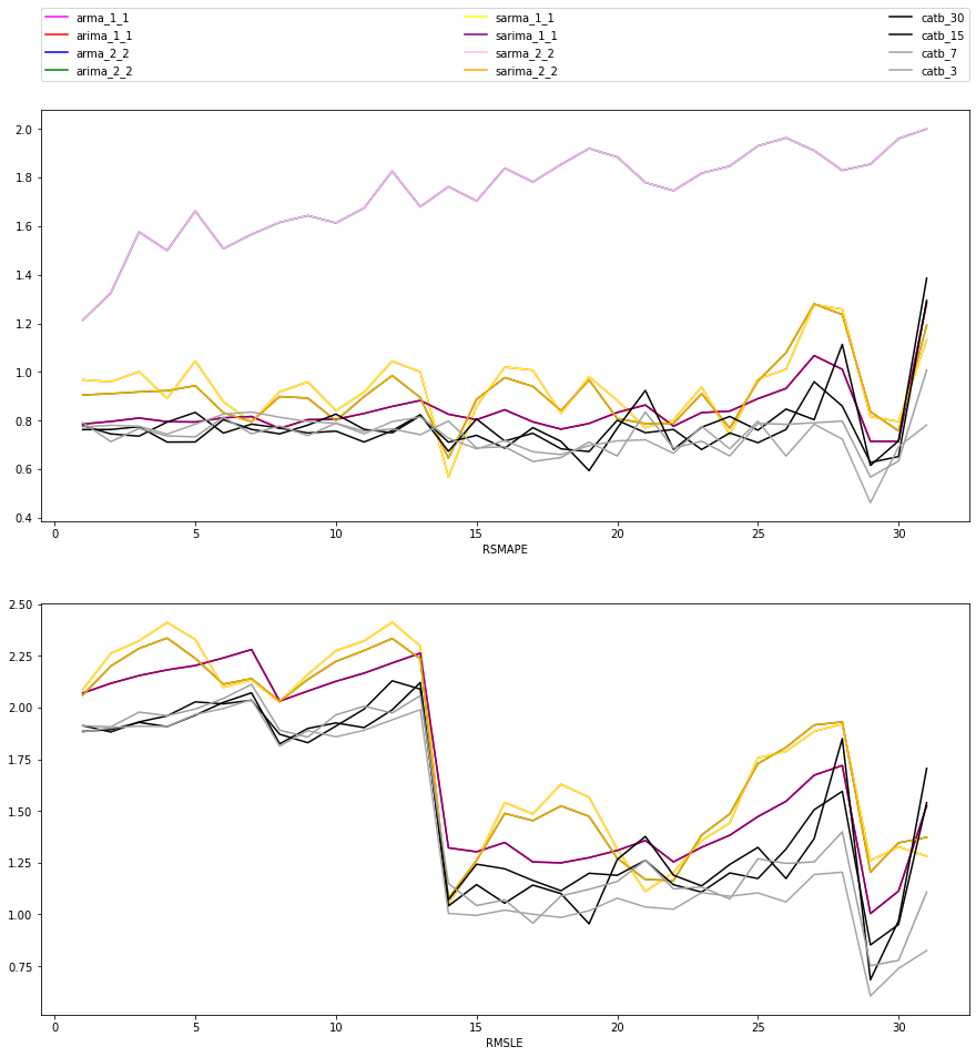
[44]:
# plot metrics for each forecast horizon for models with exogenous variables

fig, axes = plt.subplots(2,1,figsize=(15,15))
axes = axes.flatten()

colors = ['black', 'red', 'blue', 'green', 'yellow', 'purple', 'pink', 'orange']
plt.sca(axes[0])
for i, model in enumerate(fxmodels):
    plt.plot(range(1,len(smape[model])+1), smape[model], label=model, color=colors[i])
axes[0].set_xlabel("Forecast horizon")
axes[0].set_xlabel("SMAPE")
plt.legend(bbox_to_anchor=(0, 1.07, 1, 0), mode="expand", ncol=3, borderaxespad=0.)

plt.sca(axes[1])
for i, model in enumerate(fxmodels):
    plt.plot(range(1,len(rmsle[model])+1), rmsle[model], label=model, color=colors[i])
axes[1].set_xlabel("Forecast horizon")
axes[1].set_xlabel("RMSLE")
[44]:
Text(0.5, 0, 'RMSLE')
[45]:
# plot metrics for each forecast horizon for models without exogenous variables

fig, axes = plt.subplots(2,1,figsize=(15,15))
axes = axes.flatten()

colors = ['magenta', 'red', 'blue', 'green', 'yellow', 'purple', 'pink', 'orange', 'black',
          '#050505', '#a0a0a0', '#a5a5a5']
plt.sca(axes[0])
for i, model in enumerate(fmodels):
    plt.plot(range(1,len(smape[model])+1), smape[model], label=model, color=colors[i])
axes[0].set_xlabel("Forecast horizon")
axes[0].set_xlabel("RSMAPE")
plt.legend(bbox_to_anchor=(0, 1.07, 1, 0), mode="expand", ncol=3, borderaxespad=0.)

plt.sca(axes[1])
for i, model in enumerate(fmodels):
    plt.plot(range(1,len(rmsle[model])+1), rmsle[model], label=model, color=colors[i])
axes[1].set_xlabel("Forecast horizon")
axes[1].set_xlabel("RMSLE")
[45]:
Text(0.5, 0, 'RMSLE')
[46]:
# Best model for each forecast horizon including models with exogenous variables

best_df = pd.DataFrame(dict(
    MAPE=[models[np.argmin([mape[model][h] for model in models])] for h in range(30)],
    SMAPE=[models[np.argmin([smape[model][h] for model in models])] for h in range(30)],
    RMSLE=[models[np.argmin([rmsle[model][h] for model in models])] for h in range(30)],
))
best_df.index = range(1, len(best_df)+1)
best_df.index.name='Horizon'
best_df
[46]:
| MAPE | SMAPE | RMSLE | |
|---|---|---|---|
| Horizon | |||
| 1 | arma_2_2 | catb_30 | catb_3 |
| 2 | armax_2_2 | catb_7 | catb_15 |
| 3 | catb_3 | catb_15 | catb_3 |
| 4 | catb_30 | catb_30 | catb_30 |
| 5 | catb_30 | catb_30 | catb_30 |
| 6 | armax_1_1 | catb_15 | catb_3 |
| 7 | catb_3 | catb_7 | catb_15 |
| 8 | catb_3 | catb_30 | catb_3 |
| 9 | catb_15 | catb_7 | catb_15 |
| 10 | catb_3 | catb_15 | catb_3 |
| 11 | catb_30 | catb_15 | catb_3 |
| 12 | catb_3 | catb_30 | catb_3 |
| 13 | catb_3 | catb_7 | catb_3 |
| 14 | catb_3 | arma_1_1 | catb_3 |
| 15 | catb_3 | catb_3 | catb_3 |
| 16 | catb_3 | catb_30 | catb_3 |
| 17 | catb_3 | catb_7 | catb_7 |
| 18 | catb_3 | catb_7 | catb_3 |
| 19 | catb_3 | catb_30 | catb_30 |
| 20 | catb_3 | catb_7 | catb_3 |
| 21 | catb_3 | catb_3 | catb_3 |
| 22 | catb_3 | catb_3 | catb_3 |
| 23 | catb_3 | catb_15 | catb_3 |
| 24 | catb_7 | catb_7 | catb_7 |
| 25 | catb_3 | catb_15 | catb_3 |
| 26 | catb_3 | catb_3 | catb_3 |
| 27 | catb_3 | catb_3 | catb_3 |
| 28 | catb_3 | catb_3 | catb_3 |
| 29 | catb_3 | catb_3 | catb_3 |
| 30 | catb_3 | catb_7 | catb_3 |
[47]:
# Best model for each forecast horizon, limited to non-exogenous models
# To be fair, let us not use models with exogenous data from now on
# since it in practice we will not have those exogenous variables

best_df = pd.DataFrame(dict(
    MAPE=[fmodels[np.argmin([mape[model][h] for model in fmodels])] for h in range(30)],
    SMAPE=[fmodels[np.argmin([smape[model][h] for model in fmodels])] for h in range(30)],
    RMSLE=[fmodels[np.argmin([rmsle[model][h] for model in fmodels])] for h in range(30)],
))
best_df.index = range(1, len(best_df)+1)
best_df.index.name='Horizon'
best_df
[47]:
| MAPE | SMAPE | RMSLE | |
|---|---|---|---|
| Horizon | |||
| 1 | arma_2_2 | catb_30 | catb_3 |
| 2 | catb_30 | catb_7 | catb_15 |
| 3 | catb_3 | catb_15 | catb_3 |
| 4 | catb_30 | catb_30 | catb_30 |
| 5 | catb_30 | catb_30 | catb_30 |
| 6 | arma_1_1 | catb_15 | catb_3 |
| 7 | catb_3 | catb_7 | catb_15 |
| 8 | catb_3 | catb_30 | catb_3 |
| 9 | catb_15 | catb_7 | catb_15 |
| 10 | catb_3 | catb_15 | catb_3 |
| 11 | catb_30 | catb_15 | catb_3 |
| 12 | catb_3 | catb_30 | catb_3 |
| 13 | catb_3 | catb_7 | catb_3 |
| 14 | catb_3 | arma_1_1 | catb_3 |
| 15 | catb_3 | catb_3 | catb_3 |
| 16 | catb_3 | catb_30 | catb_3 |
| 17 | catb_3 | catb_7 | catb_7 |
| 18 | catb_3 | catb_7 | catb_3 |
| 19 | catb_3 | catb_30 | catb_30 |
| 20 | catb_3 | catb_7 | catb_3 |
| 21 | catb_3 | catb_3 | catb_3 |
| 22 | catb_3 | catb_3 | catb_3 |
| 23 | catb_3 | catb_15 | catb_3 |
| 24 | catb_7 | catb_7 | catb_7 |
| 25 | catb_3 | catb_15 | catb_3 |
| 26 | catb_3 | catb_3 | catb_3 |
| 27 | catb_3 | catb_3 | catb_3 |
| 28 | catb_3 | catb_3 | catb_3 |
| 29 | catb_3 | catb_3 | catb_3 |
| 30 | catb_3 | catb_7 | catb_3 |
[48]:
# Amount of times each model won
Counter(best_df.to_numpy().flatten())
[48]:
Counter({'arma_2_2': 1,
         'catb_30': 14,
         'catb_3': 51,
         'catb_7': 12,
         'catb_15': 10,
         'arma_1_1': 2})
[49]:
# Average model error
for model in np.unique(best_df.to_numpy().flatten()):
    print(model.ljust(11),
          str(np.round(np.mean(mape[model]), 3)).ljust(7),
          str(np.round(np.mean(smape[model]), 3)).ljust(7),
          str(np.round(np.mean(rmsle[model]), 3)).ljust(7),
         )
arma_1_1    3.107131938611645e+17 0.932   1.784
arma_2_2    9.762554570372993e+17 1.735   inf
catb_15     1.6025748446850157e+17 0.771   1.53
catb_3      1.3457102263941246e+17 0.739   1.389
catb_30     1.4317837800743165e+17 0.787   1.518
catb_7      1.655668907470554e+17 0.741   1.472
[50]:
# Given that, we choose catb_3
chosen_model = 'catb_3'
[51]:
true_values = tv_pv_pairs[chosen_model][0][0]
dynamic_forecast = tv_pv_pairs[chosen_model][0][1]
static_forecast = [tv_pv_pairs[chosen_model][i][1][-1] for i in range(len(tv_pv_pairs[chosen_model]))]
assert len(static_forecast) == len(dynamic_forecast)
assert len(true_values) == len(dynamic_forecast)
[52]:
final_df = dfg.copy()
final_df = final_df.iloc[-31:, [0]]
all(final_df.iloc[:,0] == true_values)
[52]:
True
[53]:
final_df['dynamic forecast'] = dynamic_forecast
final_df['static forecast'] = static_forecast
final_df['MAPE'] = mape[chosen_model]
final_df['SMAPE'] = smape[chosen_model]
final_df['RMSLE'] = rmsle[chosen_model]
[55]:
final_df
[55]:
| sales | dynamic forecast | static forecast | MAPE | SMAPE | RMSLE | |
|---|---|---|---|---|---|---|
| date | ||||||
| 2018-11-30 | 6645.2820 | 1579.885138 | 1381.737779 | 3.106174e+17 | 0.773992 | 1.880974 |
| 2018-12-01 | 5331.1780 | 1661.055884 | 1322.080279 | 2.780335e+17 | 0.780637 | 1.903091 |
| 2018-12-02 | 9951.1820 | 2295.425096 | 1365.699152 | 2.477391e+17 | 0.776961 | 1.909545 |
| 2018-12-03 | 1403.8420 | 1613.165573 | 1129.972210 | 2.892465e+17 | 0.744544 | 1.908326 |
| 2018-12-04 | 2639.6380 | 3675.007987 | 1634.538122 | 2.969482e+17 | 0.785207 | 1.966193 |
| 2018-12-05 | 1453.1360 | 1636.171255 | 1777.265236 | 2.752879e+17 | 0.826421 | 1.994819 |
| 2018-12-06 | 10.6800 | 1620.562259 | 1569.417221 | 2.902782e+17 | 0.835272 | 2.037926 |
| 2018-12-07 | 2916.5140 | 1562.400791 | 1665.965092 | 2.921562e+17 | 0.813742 | 1.813769 |
| 2018-12-08 | 7643.0410 | 1890.732618 | 1680.781767 | 4.155220e+17 | 0.796329 | 1.887826 |
| 2018-12-09 | 5470.3900 | 1524.437425 | 2014.867056 | 3.279555e+17 | 0.788983 | 1.858189 |
| 2018-12-10 | 3873.5590 | 1717.154266 | 2167.933804 | 3.777282e+17 | 0.745360 | 1.889742 |
| 2018-12-11 | 2025.0350 | 1403.989314 | 1699.883499 | 3.836697e+17 | 0.796112 | 1.940526 |
| 2018-12-12 | 0.0000 | 2138.098352 | 1556.429934 | 3.865192e+17 | 0.814682 | 1.989378 |
| 2018-12-13 | 580.9360 | 2082.946266 | 1567.840671 | 1.377434e+00 | 0.727771 | 1.005086 |
| 2018-12-14 | 3897.7140 | 1453.233810 | 1486.190010 | 1.336495e+00 | 0.683824 | 0.995467 |
| 2018-12-15 | 306.8880 | 1473.546740 | 1892.628423 | 1.374497e+00 | 0.718033 | 1.020822 |
| 2018-12-16 | 858.7020 | 1021.082402 | 1550.243866 | 1.380527e+00 | 0.671705 | 1.000987 |
| 2018-12-17 | 2027.7580 | 1769.024422 | 1608.064481 | 1.192719e+00 | 0.660408 | 0.985577 |
| 2018-12-18 | 3645.9110 | 1592.930355 | 1433.254277 | 1.414952e+00 | 0.697012 | 1.018109 |
| 2018-12-19 | 1895.9260 | 2027.992818 | 1859.294676 | 1.500920e+00 | 0.716597 | 1.078780 |
| 2018-12-20 | 377.7360 | 1229.661154 | 1513.090017 | 1.457978e+00 | 0.721132 | 1.035881 |
| 2018-12-21 | 2140.9400 | 1931.339359 | 1798.317340 | 1.298428e+00 | 0.665431 | 1.025325 |
| 2018-12-22 | 7442.0210 | 1893.638955 | 1780.265133 | 1.485212e+00 | 0.776181 | 1.105266 |
| 2018-12-23 | 1926.7760 | 2149.547163 | 1589.280811 | 1.859388e+00 | 0.683736 | 1.087954 |
| 2018-12-24 | 6233.0540 | 3050.939678 | 1611.367737 | 1.755990e+00 | 0.797701 | 1.104065 |
| 2018-12-25 | 2698.9270 | 1730.174803 | 1556.921230 | 1.981585e+00 | 0.654126 | 1.060342 |
| 2018-12-26 | 814.5940 | 1626.333499 | 2122.081710 | 2.415952e+00 | 0.785068 | 1.193049 |
| 2018-12-27 | 177.6360 | 1616.229932 | 1602.056325 | 2.462046e+00 | 0.723857 | 1.204145 |
| 2018-12-28 | 1657.3508 | 1419.269849 | 1761.322919 | 6.330888e-01 | 0.462434 | 0.606322 |
| 2018-12-29 | 2915.5340 | 1448.019351 | 1703.835757 | 9.138620e-01 | 0.692136 | 0.739220 |
| 2018-12-30 | 713.7900 | 1381.737779 | 1630.665688 | 1.284517e+00 | 0.782165 | 0.825368 |